Contents of this page is copied directly from AWS blog sites to make it Kindle friendly. Some styles & sections from these pages are removed to render this properly in 'Article Mode' of Kindle e-Reader browser. All the contents of this page is property of AWS.
Page 1|Page 2|Page 3|Page 4
ICYMI: Serverless Q4 2021
=======================
Welcome to the 15th edition of the AWS Serverless ICYMI (in case you missed it) quarterly recap. Every quarter, we share all of the most recent product launches, feature enhancements, blog posts, webinars, Twitch live streams, and other interesting things that you might have missed!
In case you missed our last ICYMI, check out what happened last quarter here.
AWS Lambda
For developers using Amazon MSK as an event source, Lambda has expanded authentication options to include IAM, in addition to SASL/SCRAM. Lambda also now supports mutual TLS authentication for Amazon MSK and self-managed Kafka as an event source.
Lambda also launched features to make it easier to operate across AWS accounts. You can now invoke Lambda functions from Amazon SQS queues in different accounts. You must grant permission to the Lambda function’s execution role and have SQS grant cross-account permissions. For developers using container packaging for Lambda functions, Lambda also now supports pulling images from Amazon ECR in other AWS accounts. To learn about the permissions required, see this documentation.
The service now supports a partial batch response when using SQS as an event source for both standard and FIFO queues. When messages fail to process, Lambda marks the failed messages and allows reprocessing of only those messages. This helps to improve processing performance and may reduce compute costs.
Lambda launched content filtering options for functions using SQS, DynamoDB, and Kinesis as an event source. You can specify up to five filter criteria that are combined using OR logic. This uses the same content filtering language that’s used in Amazon EventBridge, and can dramatically reduce the number of downstream Lambda invocations.
Amazon EventBridge
Previously, you could consume Amazon S3 events in EventBridge via CloudTrail. Now, EventBridge receives events from the S3 service directly, making it easier to build serverless workflows triggered by activity in S3. You can use content filtering in rules to identify relevant events and forward these to 18 service targets, including AWS Lambda. You can also use event archive and replay, making it possible to reprocess events in testing, or in the event of an error.
AWS Step Functions
The AWS Batch console has added support for visualizing Step Functions workflows. This makes it easier to combine these services to orchestrate complex workflows over business-critical batch operations, such as data analysis or overnight processes.
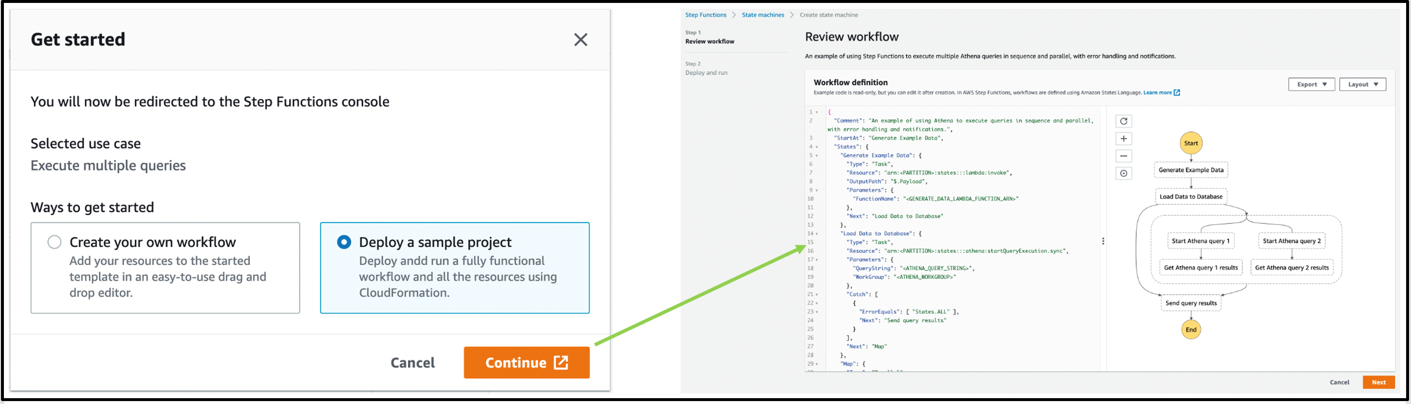
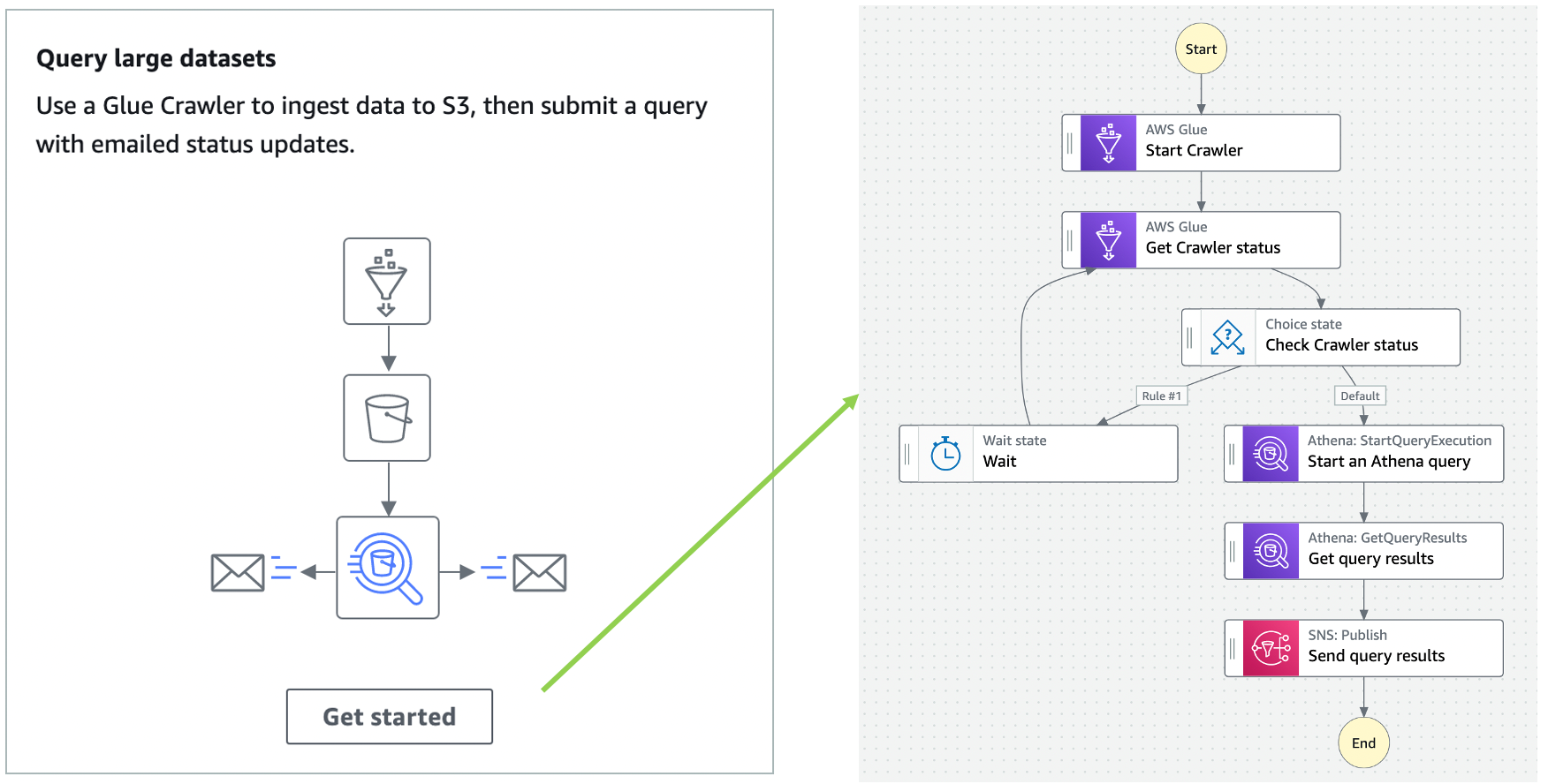
Additionally, Amazon Athena has also added console support for visualizing Step Functions workflows. This can help when building distributed data processing pipelines, allowing Step Functions to orchestrate services such as AWS Glue, Amazon S3, or Amazon Kinesis Data Firehose.
Synchronous Express Workflows now supports AWS PrivateLink. This enables you to start these workflows privately from within your virtual private clouds (VPCs) without traversing the internet. To learn more about this feature, read the What’s New post.
Amazon SNS
Amazon SNS announced support for token-based authentication when sending push notifications to Apple devices. This creates a secure, stateless communication between SNS and the Apple Push Notification (APN) service.
SNS also launched the new PublishBatch API which enables developers to send up to 10 messages to SNS in a single request. This can reduce cost by up to 90%, since you need fewer API calls to publish the same number of messages to the service.
Amazon SQS
Amazon SQS released an enhanced DLQ management experience for standard queues. This allows you to redrive messages from a DLQ back to the source queue. This can be configured in the AWS Management Console, as shown here.
Amazon DynamoDB
The NoSQL Workbench for DynamoDB is a tool to simplify designing, visualizing and querying DynamoDB tables. The tools now supports importing sample data from CSV files and exporting the results of queries.
DynamoDB announced the new Standard-Infrequent Access table class. Use this for tables that store infrequently accessed data to reduce your costs by up to 60%. You can switch to the new table class without an impact on performance or availability and without changing application code.
AWS Amplify
AWS Amplify now allows developers to override Amplify-generated IAM, Amazon Cognito, and S3 configurations. This makes it easier to customize the generated resources to best meet your application’s requirements. To learn more about the “amplify override auth” command, visit the feature’s documentation.
Similarly, you can also add custom AWS resources using the AWS Cloud Development Kit (CDK) or AWS CloudFormation. In another new feature, developers can then export Amplify backends as CDK stacks and incorporate them into their deployment pipelines.
AWS Amplify UI has launched a new Authenticator component for React, Angular, and Vue.js. Aside from the visual refresh, this provides the easiest way to incorporate social sign-in in your frontend applications with zero-configuration setup. It also includes more customization options and form capabilities.
AWS launched AWS Amplify Studio, which automatically translates designs made in Figma to React UI component code. This enables you to connect UI components visually to backend data, providing a unified interface that can accelerate development.
AWS AppSync
You can now use custom domain names for AWS AppSync GraphQL endpoints. This enables you to specify a custom domain for both GraphQL API and Realtime API, and have AWS Certificate Manager provide and manage the certificate.
To learn more, read the feature’s documentation page.
News from other services
Introducing Amazon Redshift Serverless – Run Analytics At Any Scale Without Having to Manage Data Warehouse Infrastructure
Amazon Kinesis Data Streams On-Demand – Stream Data at Scale Without Managing Capacity
AWS re:Post – A Reimagined Q&A Experience for the AWS Community
Announcing General Availability of Construct Hub and AWS Cloud Development Kit Version 2
Real-User Monitoring for Amazon CloudWatch
Introducing Amazon EMR Serverless in preview
Introducing Amazon MSK Serverless in public preview
Serverless blog posts
October
Oct 4 – Simplifying B2B integrations with AWS Step Functions Workflow Studio
Oct 6 – Operating serverless at scale: Implementing governance – Part 1
Oct 7 – Using Okta as an identity provider with Amazon MWAA
Oct 11 – Avoiding recursive invocation with Amazon S3 and AWS Lambda
Oct 12 – Operating serverless at scale: Improving consistency – Part 2
Oct 14 – Using JSONPath effectively in AWS Step Functions
Oct 14 – Accepting API keys as a query string in Amazon API Gateway
Oct 14 – Visualizing AWS Step Functions workflows from the AWS Batch console
Oct 18 – Building dynamic Amazon SNS subscriptions for auto scaling container workloads
Oct 19 – Operating serverless at scale: Keeping control of resources – Part 3
Oct 21 – Creating AWS Serverless batch processing architectures
Oct 25 – Building a difference checker with Amazon S3 and AWS Lambda
Oct 26 – Monitoring and tuning federated GraphQL performance on AWS Lambda
Oct 27 – Accelerating serverless development with AWS SAM Accelerate
Oct 28 – Creating AWS Lambda environment variables from AWS Secrets Manager
November
Nov 1 – Build workflows for Amazon Forecast with AWS Step Functions
Nov 2 – Choosing between storage mechanisms for ML inferencing with AWS Lambda
Nov 4 – Introducing cross-account Amazon ECR access for AWS Lambda
Nov 8 – Implementing header-based API Gateway versioning with Amazon CloudFront
Nov 9 – Creating static custom domain endpoints with Amazon MQ for RabbitMQ
Nov 9 – Token-based authentication for iOS applications with Amazon SNS
Nov 11 – Understanding how AWS Lambda scales with Amazon SQS standard queues
Nov 17 – Modernizing deployments with container images in AWS Lambda
Nov 18 – Deploying AWS Lambda layers automatically across multiple Regions
Nov 18 – Publishing messages in batch to Amazon SNS topics
Nov 19 – Introducing mutual TLS authentication for Amazon MSK as an event source
Nov 22 – Expanding cross-Region event routing with Amazon EventBridge
Nov 22 – Offset lag metric for Amazon MSK as an event source for Lambda
Nov 23 – Visualizing AWS Step Functions workflows from the Amazon Athena console
Nov 26 – Filtering event sources for AWS Lambda functions
December
Dec 1 – Introducing Amazon Simple Queue Service dead-letter queue redrive to source queues
Dec 13 – Using an Amazon MQ network of broker topologies for distributed microservices
Dec 27 – Building a serverless multi-player game that scales: Part 3
AWS re:Invent breakouts
AWS re:Invent was held in Las Vegas from November 29 to December 3, 2021. The Serverless DA team presented numerous breakouts, workshops and chalk talks. Rewatch all our breakout content:
What’s new in serverless
Serverless security best practices
Building real-world serverless applications with AWS SAM and Capital One
Architecting your serverless applications for hyperscale
Best practices for building interactive applications with AWS Lambda
Getting started building your first serverless application
Best practices of advanced serverless developers

We also launched an interactive serverless application at re:Invent to help customers get caffeinated!
Serverlesspresso is a contactless, serverless order management system for a physical coffee bar. The architecture comprises several serverless apps that support an ordering process from a customer’s smartphone to a real espresso bar. The customer can check the virtual line, place an order, and receive a notification when their drink is ready for pickup.

You can learn more about the architecture and download the code repo at https://serverlessland.com/reinvent2021/serverlesspresso. You can also see a video of the exhibit.
Videos

Serverless Office Hours – Tues 10 AM PT
Weekly live virtual office hours. In each session we talk about a specific topic or technology related to serverless and open it up to helping you with your real serverless challenges and issues. Ask us anything you want about serverless technologies and applications.
YouTube: youtube.com/serverlessland
Twitch: twitch.tv/aws
October
Oct 5 – Serverless Surprise! Ben Kehoe & security
Oct 12 – AWS Lambda – ARM support for Lambda functions
Oct 19 – AWS Step Functions – AWS SDK Service Integrations
Oct 20 – Using the AWS Serverless Application Model (AWS SAM) to Build Serverless Applications
Oct 26 – API Gateway – Migration tips for API keys
November
Nov 2 – pre:Invent session #1 – The serverless sessions
Nov 3 – DynamoDB Office Hours – Data Modeling with Dynobase
Nov 9 – pre:Invent session #2
Nov 16 – pre:Invent session #3
Nov 23 – pre:Invent session #4
Nov 29 – Heroes @ re:Invent part one
Nov 30 – Secret projects @ re:Invent
December
Dec 1 – Serverless leadership @ re:Invent
Dec 2 – Heroes @ re:Invent part two
Still looking for more?
The Serverless landing page has more information. The Lambda resources page contains case studies, webinars, whitepapers, customer stories, reference architectures, and even more Getting Started tutorials.
You can also follow the Serverless Developer Advocacy team on Twitter to see the latest news, follow conversations, and interact with the team.
Eric Johnson: @edjgeek
James Beswick: @jbesw
Ben Smith: @benjamin_l_s
Julian Wood: @julian_wood
Talia Nassi: @talia_nassi
Building a serverless multi-player game that scales: Part 3
=======================
This post is written by Tim Bruce, Sr. Solutions Architect, DevAx, Chelsie Delecki, Solutions Architect, DNB, and Brian Krygsman, Solutions Architect, Enterprise.
This blog series discusses building a serverless game that scales, using Simple Trivia Service:
Part 1 describes the overall architecture, how to deploy to your AWS account, and the different communication methods.
Part 2 describes adding automation to the game to help your teams scale.
This post discusses how the game scales to support concurrent users (CCU) under a load test. While this post focuses on Simple Trivia Service, you can apply the concepts to any serverless workload.
To set up the example, see the instructions in the Simple Trivia Service GitHub repo and the README.md file. This example uses services beyond AWS Free Tier and incurs charges. To remove the example from your account, see the README.md file.
Overview
Simple Trivia Service is launching at a new trivia conference. There are 200,000 registered attendees who are invited to play the game during the conference. The developers are following AWS Well-Architected best practice and load test before the launch.
Load testing is the practice of simulating user load to validate the system’s ability to scale. The focus of the load test is the game’s microservices, built using AWS Serverless services, including:
Amazon API Gateway and AWS IoT, which provide serverless endpoints, allowing users to interact with the Simple Trivia Service microservices.
AWS Lambda, which provides serverless compute services for the microservices.
Amazon DynamoDB, which provides a serverless NoSQL database for storing game data.
Preparing for load testing
Defining success criteria is one of the first steps in preparing for a load test. You use success criteria to determine how well the game meets the requirements and includes concurrent users, error rates, and response time. These three criteria help to ensure that your users have a good experience when playing your game.
Excluding one can lead to invalid assumptions about the scale of users that the game can support. If you exclude error rate goals, for example, users may encounter more errors, impacting their experience.
The success criteria used for Simple Trivia Service are:
200,000 concurrent users split across game types.
Error rates below 0.05%.
95th percentile synchronous responses under 1 second.
With these identified, you can develop dashboards to report on the targets. Dashboards allow you to monitor system metrics over the course of load tests. You can develop dashboards using Amazon CloudWatch dashboards, using custom widgets that organize and display metrics.
Common metrics to monitor include:
Error rates – total errors / total invocations.
Throttles – invocations resulting in 429 errors.
Percentage of quota usage – usage against your game’s Service Quotas.
Concurrent execution counts – maximum concurrent Lambda invocations.
Provisioned concurrency invocation rate – provisioned concurrency spillover invocation count / provisioned concurrency invocation count.
Latency – percentile-based response time, such as 90th and 95th percentiles.
Documentation and other services are also helpful during load testing. Centralized logging via Amazon CloudWatch Logs and AWS CloudTrail provide your team with operational data for the game. This data can help triage issues during testing.
System architecture documents provide key details to help your team focus their work during triage. Amazon DevOps Guru can also provide your team with potential solutions for issues. This uses machine learning to identify operational deviations and deployments and provides recommendations for resolving issues.
A load testing tool simplifies your testing, allowing you to model users playing the game. Popular load testing tools include Apache JMeter, Artillery.io Artillery, and Locust.io Locust. The load testing tool you select can act as your application client and access your endpoints directly.
This example uses Locust to load test Simple Trivia Service based on language and technical requirements. It allows you to accurately model usage and not only generate transactions. In production applications, select a tool that aligns to your team’s skills and meets your technical requirements.
You can place automation around load testing tool to reduce manual effort of running tests. Automation can include allocating environments, deploying and running test scripts, and collecting results. You can include this as part of your continuous integration/continuous delivery (CI/CD) pipeline. You can use the Distributed Load Testing on AWS solution to support Taurus-compatible load testing.
Also, document a plan, working backwards from your goals to help measure your progress. Plans typically use incremental growth of CCU, which can help you to identify constraints in your game. Use your plan while you are in development once portions of your game feature complete.
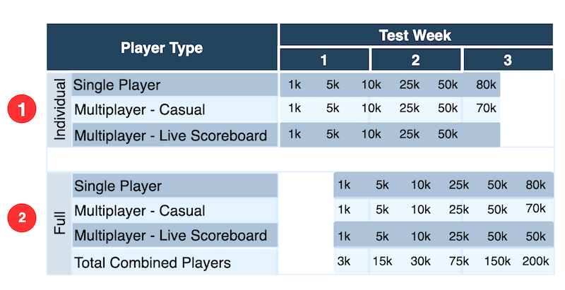
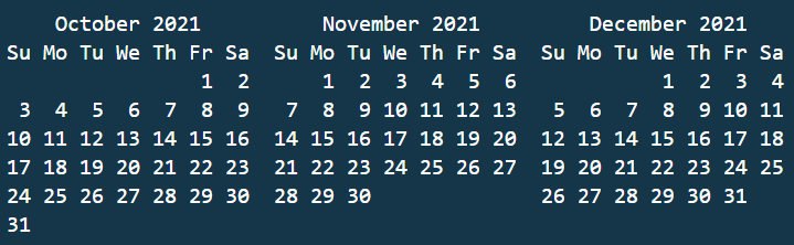
This shows an example plan for load testing Simple Trivia Service:
- Start with individual game testing to validate tests and game modes separately.
- Add in testing of the three game modes together, mirroring expected real world activity.
Finally, evaluate your load test and architecture against your AWS Customer Agreement, AWS Acceptable Use Policy, Amazon EC2 Testing Policy, and the AWS Customer Support Policy for Penetration Testing. These policies are put in place to help you to be successful in your load testing efforts. AWS Support requires you to notify them at least two weeks prior to your load test using the Simulated Events Submission Form with the AWS Management Console. This form can also be used if you have questions before your load test.
Additional help for your load test may be available on the AWS Forums, AWS re:Post, or via your account team.
Testing
After triggering a test, automation scales up your infrastructure and initializes the test users. Depending on the number of users you need and their startup behavior, this ramp-up phase can take several minutes. Similarly, when the test run is complete, your test users should ramp down. Unless you have modeled the ramp-up and ramp-down phases to match real-world behavior, exclude these phases from your measurements. If you include them, you may optimize for unrealistic user behavior.
While tests are running, let metrics normalize before drawing conclusions. Services may report data at different rates. Investigate when you find metrics that cross your acceptable thresholds. You may need to make adjustments like adding Lambda Provisioned Concurrency or changing application code to resolve constraints. You may even need to re-evaluate your requirements based on how the system performs. When you make changes, re-test to verify any changes had the impact you expected before continuing with your plan.
Finally, keep an organized record of the inputs and outputs of tests, including dashboard exports and your own observations. This record is valuable when sharing test outcomes and comparing test runs. Mark your progress against the plan to stay on track.
Analyzing and improving Simple Trivia Service performance
Running the test plan, using observability tools to measure performance, finds opportunities to tune performance bottlenecks.
In this example, during single player individual tests, the dashboards show acceptable latency values. As the test size grows, increasing read capacity for retrieving leaderboards indicates a tuning opportunity:
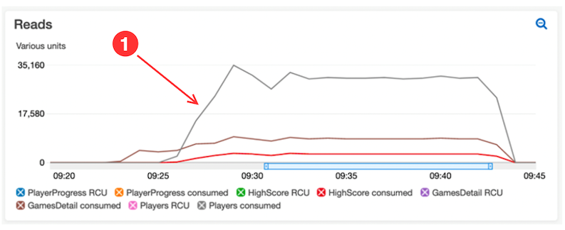
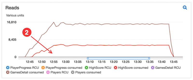
- The CloudWatch dashboard reveals that the LeaderboardGet function is leading to high consumed read capacity for the Players DynamoDB table. A process within the function is querying scores and player records with every call to load avatar URLs
- Standardizing the player avatar URL process within the code reduces reads from the table. The update improves DynamoDB reads.
Moving into the full test phase of the plan with combined game types identified additional areas for performance optimization. In one case, dashboards highlight unexpected error rates for a Lambda function. Consulting function logs and DevOps Guru to triage the behavior, these show a downstream issue with an Amazon Kinesis Data Stream:
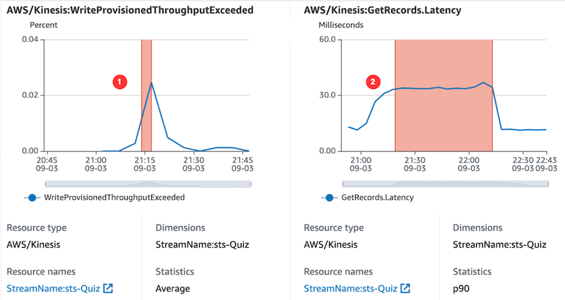
- DevOps Guru, within an insight, highlights the problem of the Kinesis:WriteProvisionedThroughputExceeded metric during our test window
- DevOps Guru also correlates that metric with the Kinesis:GetRecords.Latency metric.
DevOps Guru also links to a recommendation for Kinesis Data Streams to troubleshoot and resolve the incident with the data stream. Following this advice helps to resolve the Lambda error rates during the next test.
Load testing results
By following the plan, making incremental changes as optimizations became apparent, you can reach the goals.
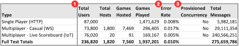
The preceding table is a summary of data from Amazon CloudWatch Lambda Insights and statistics captured from Locust:
- The test exceeded the goal of 200k CCU with a combined total of 236,820 CCU.
- Less than 0.05% error rate with a combined average of 0.010%.
- Performance goals are achieved without needing Provisioned Concurrency in Lambda.
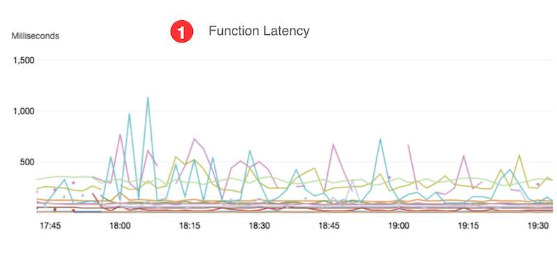
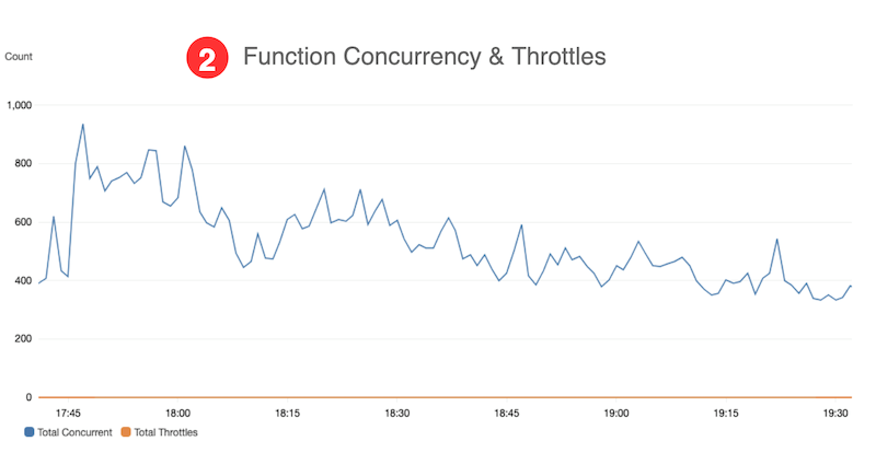
- The function latency goal of < 1 second is met, based on data from CloudWatch Lambda Insights.
- Function concurrency is below Service Quotas for Lambda during the test, based on data from our custom CloudWatch dashboard.
Conclusion
This post discusses how to perform a load test on a serverless workload. The process was used to validate a scale of Simple Trivia Service, a single- and multi-player game built using a serverless-first architecture on AWS. The results show a scale of over 220,000 CCUs while maintaining less than 1-second response time and an error rate under 0.05%.
For more serverless learning resources, visit Serverless Land.
Deep dive into NitroTPM and UEFI Secure Boot support in Amazon EC2
=======================
Contributed by Samartha Chandrashekar, Principal Product Manager Amazon EC2
At re:Invent 2021, we announced NitroTPM, a Trusted Platform Module (TPM) 2.0 and Unified Extensible Firmware Interface (UEFI) Secure Boot support in Amazon EC2. In this blog post, we’ll share additional details on how these capabilities can help further raise the security bar of EC2 deployments.
A TPM is a security device to gather and attest system state, store and generate cryptographic data, and prove platform identity. Although TPMs are traditionally discrete chips or firmware modules, their adaptation on AWS as NitroTPM preserves their security properties without affecting the agility and scalability of EC2. NitroTPM makes it possible to use TPM-dependent applications and Operating System (OS) capabilities in EC2 instances. It conforms to the TPM 2.0 specification, which makes it easy to migrate existing on-premises workloads that use TPM functionalities to EC2.
Unified Extensible Firmware Interface (UEFI) Secure Boot is a feature of UEFI that builds on EC2’s long-standing secure boot process and provides additional defense-in-depth that helps you secure software from threats that persist across reboots. It ensures that EC2 instances run authentic software by verifying the digital signature of all boot components, and halts the boot process if signature verification fails. When used with UEFI Secure Boot, NitroTPM can verify the integrity of software that boots and runs in the EC2 instance. It can measure instance properties and components as evidence that unaltered software in the correct order was used during boot. Features such as “Measured Boot” in Windows, Linux Unified Key Setup (LUKS) and dm-verity in popular Linux distributions can use NitroTPM to further secure OS launches from malware with administrative that attempt to persist across reboots.
NitroTPM derives its root-of-trust from the Nitro Security Chip and performs the same functions as a physical/discrete TPM. Similar to discrete TPMs, an immutable private and public Endorsement Key (EK) is set up inside the NitroTPM by AWS during instance creation. NitroTPM can serve as a “root-of-trust” to verify the provenance of software in the instance (e.g., NitroTPM’s EKCert as the basis for SSL certificates). Sensitive information protected by NitroTPM is made available only if the OS has booted correctly (i.e., boot measurements match expected values). If the system is tampered, keys are not released since the TPM state is different, thereby ensuring protection from malware attempting to hijack the boot process. NitroTPM can protect volume encryption keys used by full-disk encryption utilities (such as dm-crypt and BitLocker) or private keys for certificates.
NitroTPM can be used for attestation, a process to demonstrate that an EC2 instance meets pre-defined criteria, thereby allowing you to gain confidence in its integrity. It can be used to authenticate an instance requesting access to a resource (such as a service or a database) to be contingent on its health state (e.g., patching level, presence of mandated agents, etc.). For example, a private key can be “sealed” to a list of measurements of specific programs allowed to “unseal”. This makes it suited for use cases such as digital rights management to gate LDAP login, and database access on attestation. Access to AWS Key Management Service (KMS) keys to encrypt/decrypt data accessed by the instance can be made to require affirmative attestation of instance health. Anti-malware software (e.g., Windows Defender) can initiate remediation actions if attestation fails.
NitroTPM uses Platform Configuration Registers (PCR) to store system measurements. These do not change until the next boot of the instance. PCR measurements are computed during the boot process before malware can modify system state or tamper with the measuring process. These values are compared with pre-calculated known-good values, and secrets protected by NitroTPM are released only if the sequences match. PCRs are recalculated after each reboot, which ensures protection against malware aiming to hijack the boot process or persist across reboots. For example, if malware overwrites part of the kernel, measurements change, and disk decryption keys sealed to NitroTPM are not unsealed. Trust decisions can also be made based on additional criteria such as boot integrity, patching level, etc.
The workflow below shows how UEFI Secure Boot and NitroTPM work to ensure system integrity during OS startup.

To get started, you’ll need to register an Amazon Machine Image (AMI) of an Operating System that supports TPM 2.0 and UEFI Secure Boot using the register-image primitive via the CLI, API, or console. Alternatively, you can use pre-configured AMIs from AWS for both Windows and Linux to launch EC2 instances with TPM and Secure Boot. The screenshot below shows a Windows Server 2019 instance on EC2 launched with NitroTPM using its inbox TPM 2.0 drivers to recognize a TPM device.

NitroTPM and UEFI Secure Boot enables you to further raise the bar in running their workloads in a secure and trustworthy manner. We’re excited for you to try out NitroTPM when it becomes publicly available in 2022. Contact nitrotpm-interest@amazon.com for additional information.
Using an Amazon MQ network of broker topologies for distributed microservices
=======================
This post is written by Suranjan Choudhury Senior Manager SA and Anil Sharma, Apps Modernization SA.
This blog looks at ActiveMQ topologies that customers can evaluate when planning hybrid deployment architectures spanning AWS Regions and customer data centers, using a network of brokers. A network of brokers can have brokers on-premises and Amazon MQ brokers on AWS.
Distributing broker nodes across AWS and on-premises allows for messaging infrastructure to scale, provide higher performance, and improve reliability. This post also explains a topology spanning two Regions and demonstrates how to deploy on AWS.
A network of brokers is composed of multiple simultaneously active single-instance brokers or active/standby brokers. A network of brokers provides a large-scale messaging fabric in which multiple brokers are networked together. It allows a system to survive the failure of a broker. It also allows distributed messaging. Applications on remote, disparate networks can exchange messages with each other. A network of brokers helps to scale the overall broker throughput in your network, providing increased availability and performance.
Types of ActiveMQ topologies
Network of brokers can be configured in a variety of topologies – for example, mesh, concentrator, and hub and spoke. The topology depends on requirements such as security and network policies, reliability, scaling and throughput, and management and operational overheads. You can configure individual brokers to operate as a single broker or in an active/standby configuration.
Mesh topology
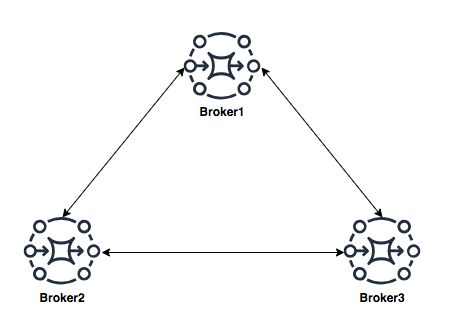
A mesh topology provides multiple brokers that are all connected to each other. This example connects three single-instance brokers, but you can configure more brokers as a mesh. The mesh topology needs subnet security group rules to be opened for allowing brokers in internal subnets to communicate with brokers in external subnets.
For scaling, it’s simpler to add new brokers for incrementing overall broker capacity. The mesh topology by design offers higher reliability with no single point of failure. Operationally, adding or deleting of nodes requires broker re-configuration and restarting the broker service.
Concentrator topology

In a concentrator topology, you deploy brokers in two (or more) layers to funnel incoming connections into a smaller collection of services. This topology allows segmenting brokers into internal and external subnets without any additional security group changes. If additional capacity is needed, you can add new brokers without needing to update other brokers’ configurations. The concentrator topology provides higher reliability with alternate paths for each broker. This enables hybrid deployments with lower operational overheads.
Hub and spoke topology

A hub and spoke topology preserves messages if there is disruption to any broker on a spoke. Messages are forwarded throughout and only the central Broker1 is critical to the network’s operation. Subnet security group rules must be opened to allow brokers in internal subnets to communicate with brokers in external subnets.
Adding brokers for scalability is constrained by the hub’s capacity. Hubs are a single point of failure and should be configured as active-standby to increase reliability. In this topology, depending on the location of the hub, there may be increased bandwidth needs and latency challenges.
Using a concentrator topology for large-scale hybrid deployments
When planning deployments spanning AWS and customer data centers, the starting point is the concentrator topology. The brokers are deployed in tiers such that brokers in each tier connect to fewer brokers at the next tier. This allows you to funnel connections and messages from a large number of producers to a smaller number of brokers. This concentrates messages at fewer subscribers:
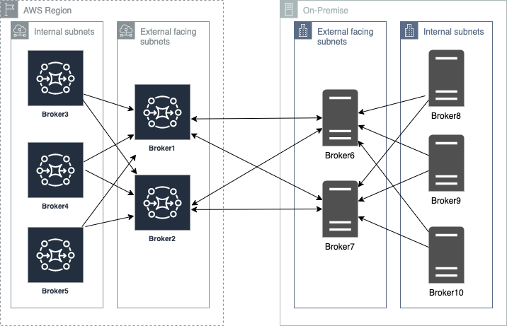
Deploying ActiveMQ brokers across Regions and on-premises
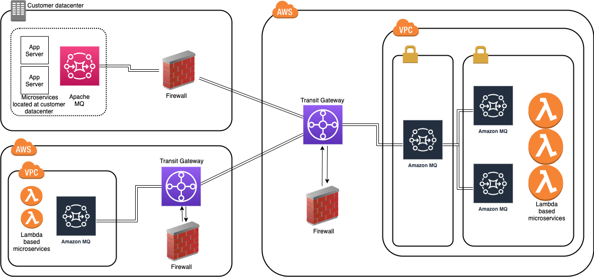
When placing brokers on-premises and in the AWS Cloud in a hybrid network of broker topologies, security and network routing are key. The following diagram shows a typical hybrid topology:

Amazon MQ brokers on premises are placed behind a firewall. They can communicate to Amazon MQ brokers through an IPsec tunnel terminating on the on-premises firewall. On the AWS side, this tunnel terminates on an AWS Transit Gateway (TGW). The TGW routes all network traffic to a firewall in AWS in a service VPC.
The firewall inspects the network traffic and routes all inspected traffic sent back to the transit gateway. The TGW, based on routing configured, sends the traffic to the Amazon MQ broker in the application VPC. This broker concentrates messages from Amazon MQ brokers hosted on AWS. The on premises brokers and the AWS brokers form a hybrid network of brokers that spans AWS and customer data center. This allows applications and services to communicate securely. This architecture exposes only the concentrating broker to receive and send messages to the broker on premises. The applications are protected from outside, non-validated network traffic.
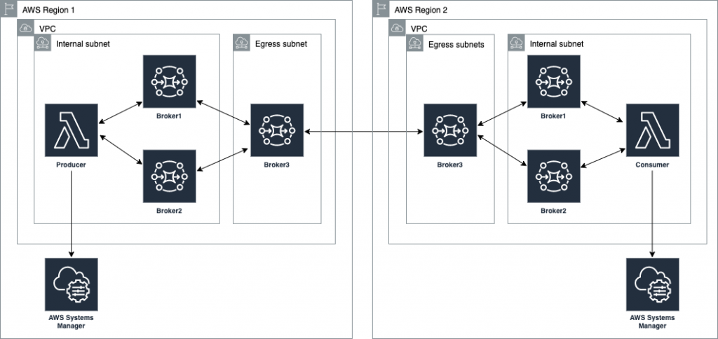
This blog shows how to create a cross-Region network of brokers. This topology removes multiple brokers in the internal subnet. However, in a production environment, you have multiple brokers’ internal subnets catering to multiple producers and consumers. This topology spans an AWS Region and an on-premises customer data center represented in a second AWS Region:
Best practices for configuring network of brokers
Client-side failover
In a network of brokers, failover transport configures a reconnect mechanism on top of the transport protocols. The configuration allows you to specify multiple URIs to connect to. An additional configuration using the randomize transport option allows for random selection of the URI when re-establishing a connection.
The example Lambda functions provided in this blog use the following configuration:
//Failover URI
failoverURI = "failover:(" + uri1 + "," + uri2 + ")?randomize=True";
Broker side failover
Dynamic failover allows a broker to receive a list of all other brokers in the network. It can use the configuration to update producer and consumer clients with this list. The clients can update to rebalance connections to these brokers.
In the broker configuration in this blog, the following configuration is set up:
<transportConnectors> <transportConnector name="openwire" updateClusterClients="true" updateClusterClientsOnRemove = "false" rebalanceClusterClients="true"/> </transportConnectors>
Network connector properties – TTL and duplex
TTL values allow messages to traverse through the network. There are two TTL values – messageTTL and consumerTTL. Another way is to set up the network TTL, which sets both the message and consumer TTL.
The duplex option allows for creating a bidirectional path between two brokers for sending and receiving messages. This blog uses the following configuration:
<networkConnector name="connector_1_to_3" networkTTL="5" uri="static:(ssl://xxxxxxxxx.mq.us-east-2.amazonaws.com:61617)" userName="MQUserName"/>
Connection pooling for producers
In the example Lambda function, a pooled connection factory object is created to optimize connections to broker:
// Create a conn factory
final ActiveMQSslConnectionFactory connFacty = new ActiveMQSslConnectionFactory(failoverURI);
connFacty.setConnectResponseTimeout(10000);
return connFacty;
// Create a pooled conn factory
final PooledConnectionFactory pooledConnFacty = new PooledConnectionFactory();
pooledConnFacty.setMaxConnections(10);
pooledConnFacty.setConnectionFactory(connFacty);
return pooledConnFacty;
Deploying the example solution
- Create an IAM role for Lambda by following the steps at https://github.com/aws-samples/aws-mq-network-of-brokers#setup-steps.
- Create the network of brokers in the first Region. Navigate to the CloudFormation console and choose Create stack:

- Provide the parameters for the network configuration section:

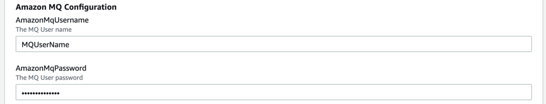
- In the Amazon MQ configuration section, configure the following parameters. Ensure that these two parameter values are the same in both Regions.

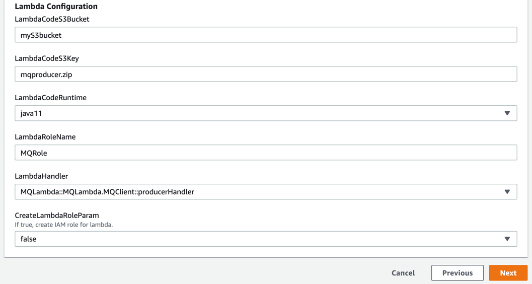
- Configure the following in the Lambda configuration section. Deploy mqproducer and mqconsumer in two separate Regions:

- Create the network of brokers in the second Region. Repeat step 2 to create the network of brokers in the second Region. Ensure that the VPC CIDR in region2 is different than the one in region1. Ensure that the user name and password are the same as in the first Region.
- Complete VPC peering and updating route tables:
- Follow the steps here to complete VPC peering between the two VPCs.
- Update the route tables in both the VPC.
- Enable DNS resolution for the peering connection.

- Configure the network of brokers and create network connectors:
- In region1, choose Broker3. In the Connections section, copy the endpoint for the openwire protocol.
- In region2 on broker3, set up the network of brokers using the networkConnector configuration element.

- Edit the configuration revision and add a new NetworkConnector within the NetworkConnectors section. Replace the uri with the URI for the broker3 in region1.
<networkConnector name="broker3inRegion2_to_ broker3inRegion1" duplex="true" networkTTL="5" userName="MQUserName" uri="static:(ssl://b-123ab4c5-6d7e-8f9g-ab85-fc222b8ac102-1.mq.ap-south-1.amazonaws.com:61617)" />
- Send a test message using the mqProducer Lambda function in region1. Invoke the producer Lambda function:
aws lambda invoke --function-name mqProducer out --log-type Tail --query 'LogResult' --output text | base64 -d 
- Receive the test message. In region2, invoke the consumer Lambda function:
aws lambda invoke --function-name mqConsumer out --log-type Tail --query 'LogResult' --output text | base64 -d 
The message receipt confirms that the message has crossed the network of brokers from region1 to region2.
Cleaning up
To avoid incurring ongoing charges, delete all the resources by following the steps at https://github.com/aws-samples/aws-mq-network-of-brokers#clean-up.
Conclusion
This blog explains the choices when designing a cross-Region or a hybrid network of brokers architecture that spans AWS and your data centers. The example starts with a concentrator topology and enhances that with a cross-Region design to help address network routing and network security requirements.
The blog provides a template that you can modify to suit specific network and distributed application scenarios. It also covers best practices when architecting and designing failover strategies for a network of brokers or when developing producers and consumers client applications.
The Lambda functions used as producer and consumer applications demonstrate best practices in designing and developing ActiveMQ clients. This includes storing and retrieving parameters, such as passwords from the AWS Systems Manager.
For more serverless learning resources, visit Serverless Land.
Implementing Auto Scaling for EC2 Mac Instances
=======================
This post is written by: Josh Bonello, Senior DevOps Architect, AWS Professional Services; Wes Fabella, Senior DevOps Architect, AWS Professional Services
Amazon Elastic Compute Cloud (Amazon EC2) is a web service that provides secure, resizable compute capacity in the cloud. The introduction of Amazon EC2 Mac now enables macOS based workloads to run in the AWS Cloud. These EC2 instances require Dedicated Hosts usage. EC2 integrates natively with Amazon CloudWatch to provide monitoring and observability capabilities.
In order to best leverage EC2 for dynamic workloads, it is a best practice to use Auto Scaling whenever possible. This will allow your workload to scale to demand, while keeping a minimal footprint during low activity periods. With Auto Scaling, you don’t have to worry about provisioning more servers to handle peak traffic or paying for more than you need.
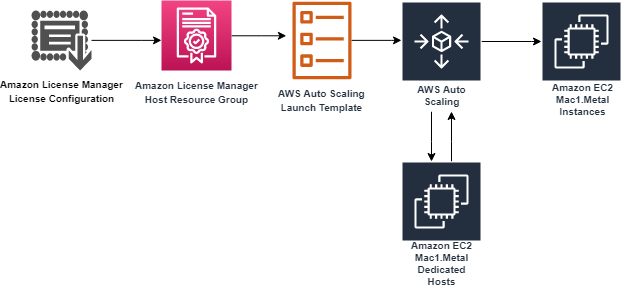
This post will discuss how to create an Auto Scaling Group for the mac1.metal instance type. We will produce an Auto Scaling Group, a Launch Template, a Host Resource Group, and a License Configuration. These resources will work together to produce the now expected behavior of standard instance types with Auto Scaling. At AWS Professional Services, we have implemented this architecture to allow the dynamic sizing of a compute fleet utilizing the mac1.metal instance type for a large customer. Depending on what should invoke the scaling mechanisms, this architecture can be easily adapted to integrate with other AWS services, such as Elastic Load Balancers (ELB). We will provide Terraform templates as part of the walkthrough. Please take special note of the costs associated with running three mac1.metal Dedicated Hosts for 24 hours.
How it works
First, we will begin in AWS License Manager and create a License Configuration. This License Configuration will be associated with an Amazon Machine Image (AMI), and can be associated with multiple AMIs. We will utilize this License Configuration as a parameter when we create a Host Resource Group. As part of defining the Launch Template, we will be referencing our Host Resource Group. Then, we will create an Auto Scaling Group based on the Launch Template.
The License Configuration will control the software licensing parameters. Normally, License Configurations are used for software licensing controls. In our case, it is only a required element for a Host Resource Group, and it handles nothing significant in our solution.
The Host Resource Group will be responsible for allocating and deallocating the Dedicated Hosts for the Mac1 instance family. An available Dedicated Host is required to launch a mac1.metal EC2 instance.
The Launch Template will govern many aspects to our EC2 Instances, including AWS Identity and Access Management (IAM) Instance Profile, Security Groups, and Subnets. These will be similar to typical Auto Scaling Group expectations. Note that, in our solution, we will use Tenancy Host Resource Group as our compute source.
Finally, we will create an Auto Scaling Group based on our Launch Template. The Auto Scaling Group will be the controller to signal when to create new EC2 Instances, create new Dedicated Hosts, and similarly terminate EC2 Instances. Unutilized Dedicated Hosts will be tracked and terminated by the Host Resource Group.
Limits
Some limits exist for this solution. To deploy this solution, a Service Quota Increase must be submitted for mac1.metal Dedicated Hosts, as the default quota is 0. Deploying the solution without this increase will result in failures when provisioning the Dedicated Hosts for the mac1.metal instances.
While testing scale-in operations of the auto scaling group, you might find that Dedicated Hosts are in “Pending” state. Mac1 documentation says “When you stop or terminate a Mac instance, Amazon EC2 performs a scrubbing workflow on the underlying Dedicated Host to erase the internal SSD, to clear the persistent NVRAM variables. If the bridgeOS software does not need to be updated, the scrubbing workflow takes up to 50 minutes to complete. If the bridgeOS software needs to be updated, the scrubbing workflow can take up to 3 hours to complete.” The Dedicated Host cannot be reused for a new scale-out operation until this scrubbing is complete. If you attempt a scale-in and a scale-out operation during testing, you might find more Dedicated Hosts than EC2 instances for your ASG as a result.
Auto Scaling Group features like dynamic scaling, health checking, and instance refresh can also cause similar side effects as a result of terminating the EC2 instances. These side effects will subside after 24 hours when a mac1 dedicate host can be released.
Building the solution
This walkthrough will utilize a Terraform template to automate the infrastructure deployment required for this solution. The following prerequisites should be met prior to proceeding with this walkthrough:
An AWS account
Terraform CLI installed
A Service Quota Increase for mac1.metal Dedicated Hosts
Before proceeding, note that the AWS resources created as part of the walkthrough have costs associated with them. Delete any AWS resources created by the walkthrough that you do not intend to use. Take special note that at the time of writing, mac1.metal Dedicated Hosts require a 24 minimum allocation time to align with Apple macOS EULA, and that mac1.metal EC2 instances are not charged separately, only the underlying Dedicated Hosts are.
Step 1: Deploy Dedicated Hosts infrastructure
First, we will do one-time setup for AWS License Manager to have the required IAM Permissions through the AWS Management Console. If you have already used License Manager, this has already been done for you. Click on “create customer managed license”, check the box, and then click on “Grant Permissions.”

To deploy the infrastructure, we will utilize a Terraform template to automate every component setup. The code is available at https://github.com/aws-samples/amazon-autoscaling-mac1metal-ec2-with-terraform. First, initialize your Terraform host. For this solution, utilize a local machine. For this walkthrough, we will assume the use of the us-west-2 (Oregon) AWS Region and the following links to help check resources will account for this.
terraform -chdir=terraform-aws-dedicated-hosts init

Then, we will plan our Terraform deployment and verify what we will be building before deployment.
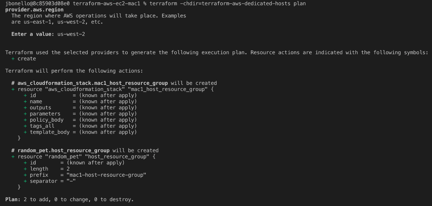
terraform -chdir=terraform-aws-dedicated-hosts plan
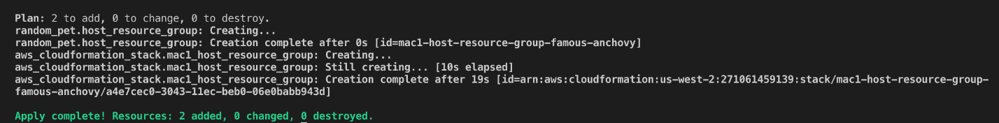
In our case, we will expect a CloudFormation Stack and a Host Resource Group.

Then, apply our Terraform deployment and verify via the AWS Management Console.
terraform -chdir=terraform-aws-dedicated-hosts apply -auto-approve

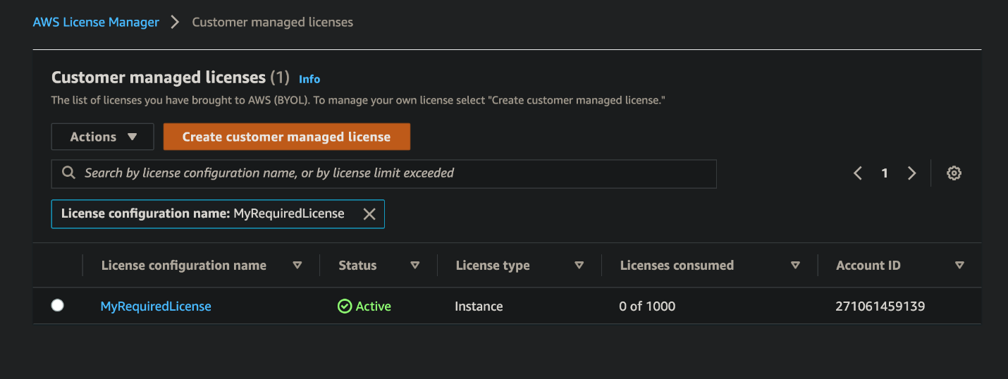
Check that the License Configuration has been made in License Manager with a name similar to MyRequiredLicense.

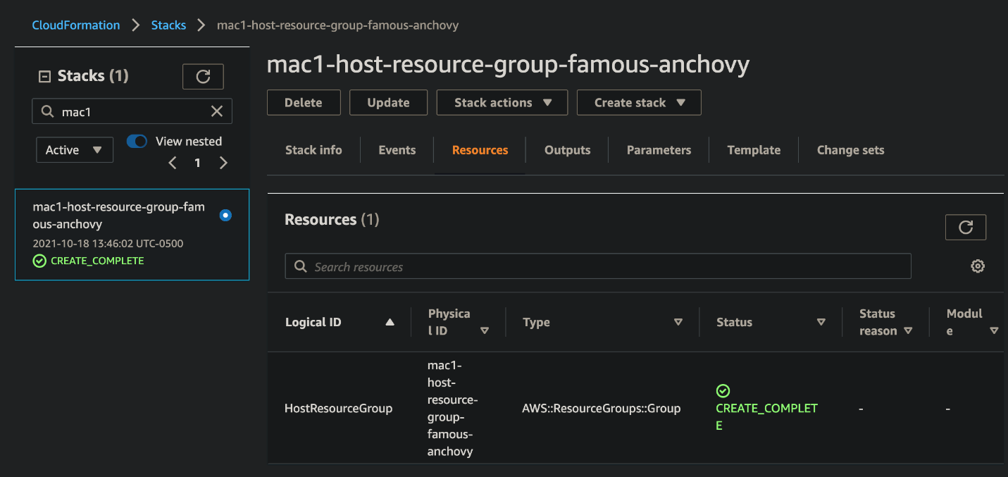
Check that the Host Resource Group has been made in the AWS Management Console. Ensure that the name is similar to mac1-host-resource-group-famous-anchovy.

Note the host resource group name in the HostResourceGroup “Physical ID” value for the next step.
Step 2: Deploy mac1.metal Auto Scaling Group
We will be taking similar steps as in Step 1 with a new component set.
Initialize your Terraform State:
terraform -chdir=terraform-aws-ec2-mac init
Then, update the following values in terraform-aws-ec2-mac/my.tfvars:
vpc_id : Check the ID of a VPC in the account where you are deploying. You will always have a “default” VPC.
subnet_ids : Check the ID of one or many subnets in your VPC.
hint: use https://us-west-2.console.aws.amazon.com/vpc/home?region=us-west-2#subnets
security_group_ids : Check the ID of a Security Group in the account where you are deploying. You will always have a “default” SG.
host_resource_group_cfn_stack_name : Use the Host Resource Group Name value from the previous step.
Then, plan your deployment using the following:
terraform -chdir=terraform-aws-ec2-mac plan -var-file="my.tfvars"
Once we’re ready to deploy, utilize Terraform to apply the following:
terraform -chdir=terraform-aws-ec2-mac apply -var-file="my.tfvars" -auto-approve
Note, this will take three to five minutes to complete.
Step 3: Verify Deployment
Check our Auto Scaling Group in the AWS Management Console for a group named something like “ec2-native-xxxx”. Verify all attributes that we care about, including the underlying EC2.

Check our Elastic Load Balancer in the AWS Management Console with a Tag key “Name” and the value of your Auto Scaling Group.
Check for the existence of our Dedicated Hosts in the AWS Management Console.
Step 4: Test Scaling Features
Now we have the entire infrastructure in place for an Auto Scaling Group to conduct normal activity. We will test with a scale-out behavior, then a scale-in behavior. We will force operations by updating the desired count of the Auto Scaling Group.
For scaling out, update the my.tfvars variable number_of_instances to three from two, and then apply our terraform template. We will expect to see one more EC2 instance for a total of three instances, with three Dedicated Hosts.
terraform -chdir=terraform-aws-ec2-mac apply -var-file="my.tfvars" -auto-approve
Then, take the steps in Step 3: Verify Deployment in order to check for expected behavior.
For scaling in, update the my.tfvars variable number_of_instances to one from three, and then apply our terraform template. We will expect your Auto Scaling Group to reduce to one active EC2 instance and have three Dedicated Hosts remaining until they are capable of being released 24 hours later.
terraform -chdir=terraform-aws-ec2-mac apply -var-file="my.tfvars" -auto-approve
Then, take the steps in Step 3: Verify Deployment in order to check for expected behavior.
Cleaning up
Complete the following steps in order to cleanup resources created by this exercise:
terraform -chdir=terraform-aws-ec2-mac destroy -var-file="my.tfvars" -auto-approve
This will take 10 to 12 minutes. Then, wait 24 hours for the Dedicated Hosts to be capable of being released, and then destroy the next template. We recommend putting a reminder on your calendar to make sure that you don’t forget this step.
terraform -chdir=terraform-aws-dedicated-hosts destroy -auto-approve
Conclusion
In this post, we created an Auto Scaling Group using mac1.metal instance types. Scaling mechanisms will work as expected with standard EC2 instance types, and the management of Dedicated Hosts is automated. This enables the management of macOS based application workloads to be automated based on the Well Architected patterns. Furthermore, this automation allows for rapid reactions to surges of demand and reclamation of unused compute once the demand is cleared. Now you can augment this system to integrate with other AWS services, such as Elastic Load Balancing, Amazon Simple Cloud Storage (Amazon S3), Amazon Relational Database Service (Amazon RDS), and more.
Review the information available regarding CloudWatch custom metrics to discover possibilities for adding new ways for scaling your system. Now we would be eager to know what AWS solution you’re going to build with the content described by this blog post! To get started with EC2 Mac instances, please visit the product page.
Introducing Amazon Simple Queue Service dead-letter queue redrive to source queues
=======================
This blog post is written by Mark Richman, a Senior Solutions Architect for SMB.
Today AWS is launching a new capability to enhance the dead-letter queue (DLQ) management experience for Amazon Simple Queue Service (SQS). DLQ redrive to source queues allows SQS to manage the lifecycle of unconsumed messages stored in DLQs.
SQS is a fully managed message queuing service that enables you to decouple and scale microservices, distributed systems, and serverless applications. Using Amazon SQS, you can send, store, and receive messages between software components at any volume without losing messages or requiring other services to be available.
To use SQS, a producer sends messages to an SQS queue, and a consumer pulls the messages from the queue. Sometimes, messages can’t be processed due to a number of possible issues. These can include logic errors in consumers that cause message processing to fail, network connectivity issues, or downstream service failures. This can result in unconsumed messages remaining in the queue.
Understanding SQS dead-letter queues (DLQs)
SQS allows you to manage the life cycle of the unconsumed messages using dead-letter queues (DLQs).
A DLQ is a separate SQS queue that one or many source queues can send messages that can’t be processed or consumed. DLQs allow you to debug your application by letting you isolate messages that can’t be processed correctly to determine why their processing didn’t succeed. Use a DLQ to handle message consumption failures gracefully.
When you create a source queue, you can specify a DLQ and the condition under which SQS moves messages from the source queue to the DLQ. This is called the redrive policy. The redrive policy condition specifies the maxReceiveCount. When a producer places messages on an SQS queue, the ReceiveCount tracks the number of times a consumer tries to process the message. When the ReceiveCount for a message exceeds the maxReceiveCount for a queue, SQS moves the message to the DLQ. The original message ID is retained.
For example, a source queue has a redrive policy with maxReceiveCount set to 5. If the consumer of the source queue receives a message 6, without successfully consuming it, SQS moves the message to the dead-letter queue.
You can configure an alarm to alert you when any messages are delivered to a DLQ. You can then examine logs for exceptions that might have caused them to be delivered to the DLQ. You can analyze the message contents to diagnose consumer application issues. Once the issue has been resolved and the consumer application recovers, these messages can be redriven from the DLQ back to the source queue to process them successfully.
Previously, this required dedicated operational cycles to review and redrive these messages back to their source queue.
DLQ redrive to source queues
DLQ redrive to source queues enables SQS to manage the second part of the lifecycle of unconsumed messages that are stored in DLQs. Once the consumer application is available to consume the failed messages, you can now redrive the messages from the DLQ back to the source queue. You can optionally review a sample of the available messages in the DLQ. You redrive the messages using the Amazon SQS console. This allows you to more easily recover from application failures.
Using redrive to source queues
To show how to use the new functionality there is an existing standard source SQS queue called MySourceQueue.
SQS does not create DLQs automatically. You must first create an SQS queue and then use it as a DLQ. The DLQ must be in the same region as the source queue.
Create DLQ
- Navigate to the SQS Management Console and create a standard SQS queue for the DLQ called MyDLQ. Use the default configuration. Refer to the SQS documentation for instructions on creating a queue.
- Navigate to MySourceQueue and choose Edit.
- Navigate to the Dead-letter queue section and choose Enabled.
- Select the Amazon Resource Name (ARN) of the MyDLQ queue you created previously.
- You can configure the number of times that a message can be received before being sent to a DLQ by setting Set Maximum receives to a value between 1 and 1,000. For this demo enter a value of 1 to immediately drive messages to the DLQ.
- Choose Save.

Configure source queue with DLQ
The console displays the Details page for the queue. Within the Dead-letter queue tab, you can see the Maximum receives value and DLQ ARN.

DLQ configuration
Send and receive test messages
You can send messages to test the functionality in the SQS console.
- Navigate to MySourceQueue and choose Send and receive messages
- Send a number of test messages by entering the message content in Message body and choosing Send message.

Send and receive messages
- Navigate to the Receive messages section where you can see the number of messages available.
- Choose Poll for messages. The Maximum message count is set to 10 by default If you sent more than 10 test messages, poll multiple times to receive all the messages.

Poll for messages
All the received messages are sent to the DLQ because the maxReceiveCount is set to 1. At this stage you would normally review the messages. You would determine why their processing didn’t succeed and resolve the issue.
Redrive messages to source queue
Navigate to the list of all queues and filter if required to view the DLQ. The queue displays the approximate number of messages available in the DLQ. For standard queues, the result is approximate because of the distributed architecture of SQS. In most cases, the count should be close to the actual number of messages in the queue.

Messages available in DLQ
- Select the DLQ and choose Start DLQ redrive.

DLQ redrive
SQS allows you to redrive messages either to their source queue(s) or to a custom destination queue.
- Choose to Redrive to source queue(s), which is the default.
Redrive has two velocity control settings.
System optimized sends messages back to the source queue as fast as possible
Custom max velocity allows SQS to redrive messages with a custom maximum rate of messages per second. This feature is useful for minimizing the impact to normal processing of messages in the source queue.
You can optionally inspect messages prior to redrive.
To redrive the messages back to the source queue, choose DLQ redrive.

DLQ redrive
The Dead-letter queue redrive status panel shows the status of the redrive and percentage processed. You can refresh the display or cancel the redrive.

Dead-letter queue redrive status
Once the redrive is complete, which takes a few seconds in this example, the status reads Successfully completed.

Redrive status completed
Navigate back to the source queue and you can see all the messages are redriven back from the DLQ to the source queue.

Messages redriven from DLQ to source queue
Conclusion
Dead-letter queue redrive to source queues allows you to effectively manage the life cycle of unconsumed messages stored in dead-letter queues. You can build applications with the confidence that you can easily examine unconsumed messages, recover from errors, and reprocess failed messages.
You can redrive messages from their DLQs to their source queues using the Amazon SQS console.
Dead-letter queue redrive to source queues is available in all commercial regions, and coming soon to GovCloud.
To get started, visit https://aws.amazon.com/sqs/
For more serverless learning resources, visit Serverless Land.
Announcing winners of the AWS Graviton Challenge Contest and Hackathon
=======================
At AWS, we are constantly innovating on behalf of our customers so they can run virtually any workload, with optimal price and performance. Amazon EC2 now includes more than 475 instance types that offer a choice of compute, memory, networking, and storage to suit your workload needs. While we work closely with our silicon partners to offer instances based on their latest processors and accelerators, we also drive more choice for our customers by building our own silicon.
The AWS Graviton family of processors were built as part of that silicon innovation initiative with the goal of pushing the price performance envelope for a wide variety of customer workloads in EC2. We now have 12 EC2 instance families powered by AWS Graviton2 processors – general purpose (M6g, M6gd), burstable (T4g), compute optimized (C6g, C6gd, C6gn), memory optimized (R6g, R6gd, X2gd), storage optimized (Im4gn, Is4gen), and accelerated computing (G5g) available globally across 23 AWS Regions. We also announced the preview of Amazon EC2 C7g instances powered by the latest generation AWS Graviton3 processors that will provide the best price performance for compute-intensive workloads in EC2. Thousands of customers, including Discovery, DIRECTV, Epic Games, and Formula 1, have realized significant price performance benefits with AWS Graviton-based instances for a broad range of workloads. This year, AWS Graviton-based instances also powered much of Amazon Prime Day 2021 and supported 12 core retail services during the massive 2-day online shopping event.
To make it easy for customers to adopt Graviton-based instances, we launched a program called the Graviton Challenge. Working with customers, we saw that many successful adoptions of Graviton-based instances were the result of one or two developers taking a single workload and spending a few days to benchmark the price performance gains with Graviton2-based instances, before scaling it to more workloads. The Graviton Challenge provides a step-by-step plan that developers can follow to move their first workload to Graviton-based instances. With the Graviton Challenge, we also launched a Contest (US-only), and then a Hackathon (global), where developers could compete for prizes by building new applications or moving existing applications to run on Graviton2-based instances. More than a thousand participants, including enterprises, startups, individual developers, open-source developers, and Arm developers, registered and ran a variety of applications on Graviton-based instances with significant price performance benefits. We saw some fantastic entries and usage of Graviton2-based instances across a variety of use cases and want to highlight a few.
The Graviton Challenge Contest winners:
Best Adoption – Enterprise and Most Impactful Adoption: VMware vRealize SRE team, who migrated 60 micro-services written in Java, Rust, and Golang to Graviton2-based general purpose and compute optimized instances and realized up to 48% latency reduction and 22% cost savings.
Best Adoption – Startup: Kasm Technologies, who realized up to 48% better performance and 25% potential cost savings for its container streaming platform built on C/C++ and Python.
Best New Workload adoption: Dustin Wilson, who built a dynamic tile server based on Golang and running on Graviton2-based memory-optimized instances that helps analysts query large geospatial datasets and benchmarked up to 1.8x performance gains over comparable x86-based instances.
Most Innovative Adoption: Loroa, an application that translates any given text into spoken words from one language into multiple other languages using Graviton2-based instances, Amazon Polly, and Amazon Translate.
If you are attending AWS re:Invent 2021 in person, you can hear more details on their Graviton adoption experience by attending the CMP213: Lessons learned from customers who have adopted AWS Graviton chalk talk.
Winners for the Graviton Challenge Hackathon:
Best New App: PickYourPlace, an open-source based data analytics platform to help users select a place to live based on property value, safety, and accessibility.
Best Migrated App: Genie, an image credibility checker based on deep learning that makes predictions on photographic and tampered confidence of an image.
Highest Potential Impact: Welly Tambunan, who’s also an AWS Community Builder, for porting big data platforms Spark, Dremio, and AirByte to Graviton2 instances so developers can leverage it to build big data capabilities into their applications.
Most Creative Use Case: OXY, a low-cost custom Oximeter with mobile and web apps that enables continuous and remote monitoring to prevent deaths due to Silent Hypoxia.
Best Technical Implementation: Apollonia Bot that plays songs, playlists, or podcasts on a Discord voice channel, so users can listen to it together.
It’s been incredibly exciting to see the enthusiasm and benefits realized by our customers. We are also thankful to our judges – Patrick Moorhead from Moor Insights & Strategy, James Governor from RedMonk, and Jason Andrews from Arm, for their time and effort.
In addition to EC2, several AWS services for databases, analytics, and even serverless support options to run on Graviton-based instances. These include Amazon Aurora, Amazon RDS, Amazon MemoryDB, Amazon DocumentDB, Amazon Neptune, Amazon ElastiCache, Amazon OpenSearch, Amazon EMR, AWS Lambda, and most recently, AWS Fargate. By using these managed services on Graviton2-based instances, customers can get significant price performance gains with minimal or no code changes. We also added support for Graviton to key AWS infrastructure services such as Elastic Beanstalk, Amazon EKS, Amazon ECS, and Amazon CloudWatch to help customers build, run, and scale their applications on Graviton-based instances. Additionally, a large number of Linux and BSD-based operating systems, and partner software for security, monitoring, containers, CI/CD, and other use cases now support Graviton-based instances and we recently launched the AWS Graviton Ready program as part of the AWS Service Ready program to offer Graviton-certified and validated solutions to customers.
Congrats to all of our Contest and Hackathon winners! Full list of the Contest and Hackathon winners is available on the Graviton Challenge page.
P.S.: Even though the Contest and Hackathon have ended, developers can still access the step-by-step plan on the Graviton Challenge page to move their first workload to Graviton-based instances.
Filtering event sources for AWS Lambda functions
=======================
This post is written by Heeki Park, Principal Specialist Solutions Architect – Serverless.
When an AWS Lambda function is configured with an event source, the Lambda service triggers a Lambda function for each message or record. The exact behavior depends on the choice of event source and the configuration of the event source mapping. The event source mapping defines how the Lambda service handles incoming messages or records from the event source.
Today, AWS announces the ability to filter messages before the invocation of a Lambda function. Filtering is supported for the following event sources: Amazon Kinesis Data Streams, Amazon DynamoDB Streams, and Amazon SQS. This helps reduce requests made to your Lambda functions, may simplify code, and can reduce overall cost.
Overview
Consider a logistics company with a fleet of vehicles in the field. Each vehicle is enabled with sensors and 4G/5G connectivity to emit telemetry data into Kinesis Data Streams:
In one scenario, they use machine learning models to infer the health of vehicles based on each payload of telemetry data, which is outlined in example 2 on the Lambda pricing page.
In another scenario, they want to invoke a function, but only when tire pressure is low on any of the tires.
If tire pressure is low, the company notifies the maintenance team to check the tires when the vehicle returns. The process checks if the warehouse has enough spare replacements. Optionally, it notifies the purchasing team to buy additional tires.
The application responds to the stream of incoming messages and runs business logic if tire pressure is below 32 psi. Each vehicle in the field emits telemetry as follows:
{
"time": "2021-11-09 13:32:04",
"fleet_id": "fleet-452",
"vehicle_id": "a42bb15c-43eb-11ec-81d3-0242ac130003",
"lat": 47.616226213162406,
"lon": -122.33989110734133,
"speed": 43,
"odometer": 43519,
"tire_pressure": [41, 40, 31, 41],
"weather_temp": 76,
"weather_pressure": 1013,
"weather_humidity": 66,
"weather_wind_speed": 8,
"weather_wind_dir": "ne"
}
To process all messages from a fleet of vehicles, you configure a filter matching the fleet id in the following example. The Lambda service applies the filter pattern against the full payload that it receives.
The schema of the payload for Kinesis is shown under the “kinesis” attribute in the example Kinesis record event. When building filters for Kinesis, you filter the payload under the “data” attribute. The schema of the payload for DynamoDB streams is shown in the array of records in the example DynamoDB streams record event. When working with DynamoDB streams, you filter the payload under the “dynamodb” attribute. The schema of the payload for SQS is shown in the array of records in the example SQS message event. When working with SQS, you filter the payload under the “body” attribute:
{
"data": {
"fleet_id": ["fleet-452"]
}
}
To process all messages associated with a specific vehicle, configure a filter on only that vehicle id. The fleet id is kept in the example to show that it matches on both of those filter criteria:
{
"data": {
"fleet_id": ["fleet-452"],
"vehicle_id": ["a42bb15c-43eb-11ec-81d3-0242ac130003"]
}
}
To process all messages associated with that fleet but only if tire pressure is below 32 psi, you configure the following rule pattern. This pattern searches the array under tire_pressure to match values less than 32:
{
"data": {
"fleet_id": ["fleet-452"],
"tire_pressure": [{"numeric": ["<", 32]}]
}
}
To create the event source mapping with this filter criteria with an AWS CLI command, run the following command.
aws lambda create-event-source-mapping \
--function-name fleet-tire-pressure-evaluator \
--batch-size 100 \
--starting-position LATEST \
--event-source-arn arn:aws:kinesis:us-east-1:0123456789012:stream/fleet-telemetry \
--filter-criteria '{"Filters": [{"Pattern": "{\"tire_pressure\": [{\"numeric\": [\"<\", 32]}]}"}]}'
For the CLI, the value for Pattern in the filter criteria requires the double quotes to be escaped in order to be properly captured.
Alternatively, to create the event source mapping with this filter criteria with an AWS Serverless Application Model (AWS SAM) template, use the following snippet.
Events:
TirePressureEvent:
Type: Kinesis
Properties:
BatchSize: 100
StartingPosition: LATEST
Stream: "arn:aws:kinesis:us-east-1:0123456789012:stream/fleet-telemetry"
FilterCriteria:
Filters:
- Pattern: "{\"data\": {\"tire_pressure\": [{\"numeric\": [\"<\", 32]}]}}"
For the AWS SAM template, the value for Pattern in the filter criteria does not require escaped double quotes.
For more information on how to create filters, refer to examples of event pattern rules in EventBridge, as Lambda filters messages in the same way.
Reducing costs with event filtering
By configuring the event source with this filter criteria, you can reduce the number of messages that are used to invoke your Lambda function.
Using the example from the Lambda pricing page, with a fleet of 10,000 vehicles in the field, each is emitting telemetry once an hour. Each month, the vehicles emit 10,000 * 24 * 31 = 7,440,000 messages, which trigger the same number of Lambda invocations. You configure the function with 256 MB of memory and the average duration of the function is 100 ms. In this example, vehicles emit low-pressure telemetry once every 31 days.
Without filtering, the cost of the application is:
Monthly request charges → 7.44M * $0.20/million = $1.49
Monthly compute duration (seconds) → 7.44M * 0.1 seconds = 0.744M seconds
Monthly compute (GB-s) → 256MB/1024MB * 0.744M seconds = 0.186M GB-s
Monthly compute charges → 0.186M GB-s * $0.0000166667 = $3.10
Monthly total charges = $1.49 + $3.10 = $4.59
With filtering, the cost of the application is:
Monthly request charges → (7.44M / 31)* $0.20/million = $0.05
Monthly compute duration (seconds) → (7.44M / 31) * 0.1 seconds = 0.024M seconds
Monthly compute (GB-s) → 256MB/1024MB * 0.024M seconds = 0.006M GB-s
Monthly compute charges → 0.006M GB-s * $0.0000166667 = $0.10
Monthly total charges = $0.05 + $0.10 = $0.15
By using filtering, the cost is reduced from $4.59 to $0.15, a 96.7% cost reduction.
Designing and implementing event filtering
In addition to reducing cost, the functions now operate more efficiently. This is because they no longer iterate through arrays of messages to filter out messages. The Lambda service filters the messages that it receives from the source before batching and sending them as the payload for the function invocation. This is the order of operations:

Event flow with filtering
As you design filter criteria, keep in mind a few additional properties. The event source mapping allows up to five patterns. Each pattern can be up to 2048 characters. As the Lambda service receives messages and filters them with the pattern, it fills the batch per the normal event source behavior.
For example, if the maximum batch size is set to 100 records and the maximum batching window is set to 10 seconds, the Lambda service filters and accumulates records in a batch until one of those two conditions is satisfied. In the case where 100 records that meet the filter criteria come during the batching window, the Lambda service triggers a function with those filtered 100 records in the payload.
If fewer than 100 records meeting the filter criteria arrive during the batch window, Lambda triggers a function with the filtered records that came during the batch window at the end of the 10-second batch window. Be sure to configure the batch window to match your latency requirements.
The Lambda service ignores filtered messages and treats them as successfully processed. For Kinesis Data Streams and DynamoDB Streams, the iterator advances past the records that were sent via the event source mapping.
For SQS, the messages are deleted from the queue without any additional processing. With SQS, be sure that the messages that are filtered out are not required. For example, you have an Amazon SNS topic with multiple SQS queues subscribed. The Lambda functions consuming each of those SQS queues process different subsets of messages. You could use filters on SNS but that would require the message publisher to add attributes to the messages that it sends. You could instead use filters on the event source mapping for SQS. Now the publisher does not need to make any changes, as the filter is applied on the messages payload directly.
Conclusion
Lambda now supports the ability to filter messages based on a criteria that you define. This can reduce the number of messages that your functions process, may reduce cost, and can simplify code.
You can now build applications for specific use cases that use only a subset of the messages that flow through your event-driven architectures. This can help optimize the compute efficiency of your functions.
Learn more about this capability in our AWS Lambda Developer Guide.
Using EC2 Auto Scaling predictive scaling policies with Blue/Green deployments
=======================
This post is written by Ankur Sethi, Product Manager for EC2.
Amazon EC2 Auto Scaling allows customers to realize the elasticity benefits of AWS by automatically launching and shutting down instances to match application demand. Earlier this year we introduced predictive scaling, a new EC2 Auto Scaling policy that predicts demand and proactively scales capacity, resulting in better availability of your applications (if you are new to predictive scaling, I suggest you read this blog post before proceeding). In this blog, I will walk you through how to use a new feature, predictive scaling custom metrics, to configure predictive scaling for an application that follows a Blue/Green deployment strategy.
Blue/Green Deployment using Auto Scaling groups
The fundamental idea behind Blue/Green deployment is to shift traffic between two environments that are running different versions of your application. The Blue environment represents your current application version serving production traffic. In parallel, the Green environment is staged running the newer version. After the Green environment is ready and tested, production traffic is redirected from Blue to Green either all at once or in increments, similar to canary deployments. At the end of the load transfer, you can either terminate the Blue Auto Scaling group or reuse it to stage the next version update. Irrespective of the approach, when a new Auto Scaling group is created as part of Blue/Green deployment, EC2 Auto Scaling, and in turn predictive scaling, does not know that this new Auto Scaling group is running the same application that the Blue one was. Predictive scaling needs a minimum of 24 hours of historical metric data and up to 14 days for the most accurate results, neither of which the new Auto Scaling group has when the Blue/Green deployment is initiated. This means that if you frequently conduct Blue/Green deployments, predictive scaling regularly pauses for at least 24 hours, and you may experience less optimal forecasts after each deployment.
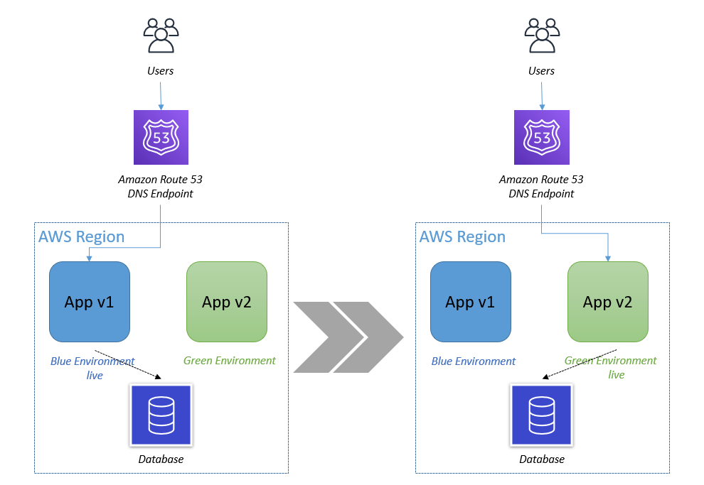
Figure 1. In Blue/Green deployment you have two Auto Scaling groups running different versions of an application. You switch production traffic from Blue to Green to make the updated version public.
How to retain your application load history using predictive scaling custom metrics
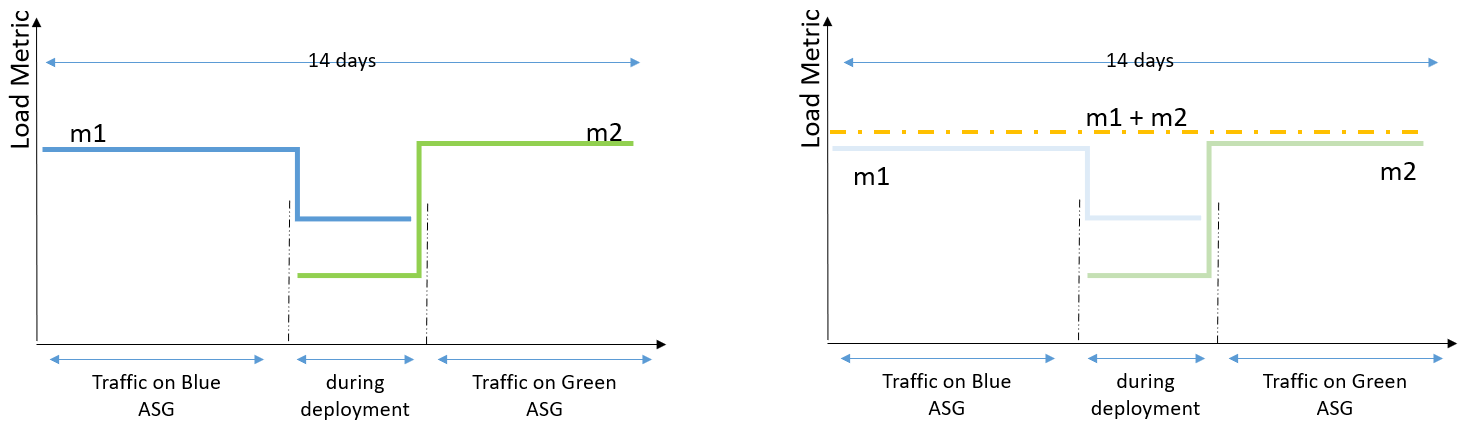
To make predictive scaling work for Blue/Green deployment scenarios, we need to aggregate load metrics from both Blue and Green environments before using it to forecast capacity as depicted in the following illustration. The key benefit of using the aggregated metric is that, throughout the Blue/Green deployment, predictive scaling can continue to forecast load correctly without a pause, and it can retain the entire 14 days of data to provide the best predictions. For example, if your application observes different patterns during a weekday vs. a weekend, predictive scaling will be able to retain knowledge of that pattern after the deployment.

Figure 2. The aggregated metrics of Blue and Green Auto Scaling groups give you the total load traffic of an application. Predictive scaling gives most accurate forecasts when based on last 14 days of history.
Example
Let’s explore this solution with an example. I created a sample application and load simulation infrastructure that you can use to follow along by deploying this example AWS CloudFormation Stack in your account. This example deploys two Auto Scaling groups: ASG-myapp-v1 (Blue) and ASG-myapp-v2 (Green) to run a sample application. Only ASG-myapp-v1 is attached to a load balancer and has recurring requests generated for its application. I have applied a target tracking policy and predictive scaling policy to maintain CPU utilization at 25%. You should keep this Auto Scaling group running for at least 24 hours before proceeding with the rest of the example to have enough load generated for predictive scaling to start forecasting.
ASG-myapp-v2 does not have any requests generated of its own. In the following sections, to highlight how metric aggregation works, I will apply a predictive scaling policy to it using Custom Metric configurations aggregating CPU Utilization metrics of both Auto Scaling groups. I’ll then verify if the forecasts are generated for ASG-myapp-v2 based on the aggregated metrics.
As part of your Blue/Green deployment approach, if you alternate between exactly two Auto Scaling groups, then you can use simple math expressions such as SUM (m1, m2) where m1 and m2 are metrics for each Auto Scaling group. However, if you create new Auto Scaling groups for each deployment, then you need to refer to the metrics of all the Auto Scaling groups that were used to run the application in the last 14 days. You can simplify this task by following a naming convention for your Auto Scaling groups and leveraging the Search expression to select the required metrics. The naming convention is ASG-myapp-vx where we name the new Auto Scaling group according to the version number (ASG-myapp-v1 → ASG-myapp-v2 and so on). Using SEARCH(‘ {Namespace, DimensionName1, DimensionName2} SearchTerm’, ‘Statistic’, Period) expression I can identify the metrics of all the Auto Scaling groups that follow the name according to the SearchTerm. I can then aggregate the metrics by appending another expression. The final expression should look like SUM(SEARCH(…).
Step 1: Apply predictive scaling policy to Green Auto Scaling group ASG-myapp-v2 with custom metrics
To generate forecasts, the predictive scaling algorithm needs three metrics as input: a load metric that represents total demand on an Auto Scaling group, the number of instances that represents the capacity of the Auto Scaling groups, and a scaling metric that represents the average utilization of the instances in the Auto Scaling groups.
Here is how it would work with CPU Utilization metrics. First, create a scaling configuration file where you define the metrics, target value, and the predictive scaling mode for your policy.
cat predictive-scaling-policy-cpu.json
{
"MetricSpecifications": [
{
"CustomizedScalingMetricSpecification": {
},
"CustomizedLoadMetricSpecification": {
},
"CustomizedCapacityMetricSpecification": {
}
}
],
"Mode": "ForecastOnly"
}
EoF
I’ll elaborate on each of these metric specifications separately in the following sections. You can download the complete JSON file in GitHub.
Customized Load Metric Specification: You can aggregate the demand across your Auto Scaling groups by using the SUM expression. The demand forecasts are generated every hour, so this metric has to be aggregated with a time period of 3600 seconds.
"CustomizedLoadMetricSpecification": {
"MetricDataQueries": [
{
"Id": "load_sum",
"Expression": "SUM(SEARCH('{AWS/EC2,AutoScalingGroupName} MetricName=\"CPUUtilization\" ASG-myapp', 'Sum', 3600))"
}
]
}
Customized Capacity Metric Specification: Your customized capacity metric represents the total number of instances across your Auto Scaling groups. Similar to the load metric, the aggregation across Auto Scaling groups is done by using the SUM expression. Note that this metric has to follow a 300 seconds interval period.
"CustomizedCapacityMetricSpecification": {
"MetricDataQueries": [
{
"Id": "capacity_sum",
"Expression": "SUM(SEARCH('{AWS/AutoScaling,AutoScalingGroupName} MetricName=\"GroupInServiceIntances\" ASG-myapp', 'Average', 300))"
}
]
}
Customized Scaling Metric Specification: Your customized scaling metric represents the average utilization of the instances across your Auto Scaling groups. We cannot simply SUM the scaling metric of each Auto Scaling group as the utilization is an average metric that depends on the capacity and demand of the Auto Scaling group. Instead, we need to find the weighted average unit load (Load Metric/Capacity). To do so, we will use an expression: Sum(load)/Sum(capacity). Note that this metric also has to follow a 300 seconds interval period.
"CustomizedScalingMetricSpecification": {
"MetricDataQueries": [
{
"Id": "capacity_sum",
"Expression": "SUM(SEARCH('{AWS/AutoScaling,AutoScalingGroupName} MetricName=\"GroupInServiceIntances\" ASG-myapp', 'Average', 300))"
“ReturnData”: “False”
},
{
"Id": "load_sum",
"Expression": "SUM(SEARCH('{AWS/EC2,AutoScalingGroupName} MetricName=\"CPUUtilization\" ASG-myapp', 'Sum', 300))"
“ReturnData”: “False”
},
{
"Id": "weighted_average",
"Expression": "load_sum / capacity_sum”
}
]
}
Once you have created the configuration file, you can run the following CLI command to add the predictive scaling policy to your Green Auto Scaling group.
aws autoscaling put-scaling-policy \
--auto-scaling-group-name "ASG-myapp-v2" \
--policy-name "CPUUtilizationpolicy" \
--policy-type "PredictiveScaling" \
--predictive-scaling-configuration file://predictive-scaling-policy-cpu.json
Instantaneously, the forecasts will be generated for the Green Auto Scaling group (My-ASG-v2) as if this new Auto Scaling group has been running the application. You can validate this using the predictive scaling forecasts API. You can also use the console to review forecasts by navigating to the Amazon EC2 Auto Scaling console, selecting the Auto Scaling group that you configured with predictive scaling, and viewing the predictive scaling policy located under the Automatic Scaling section of the Auto Scaling group details view.
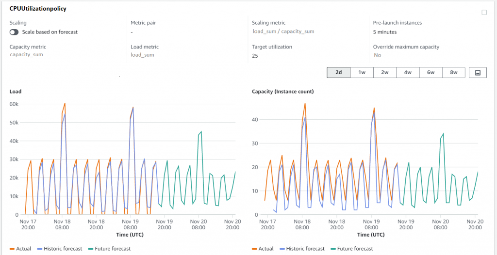
Figure 3. EC2 Auto Scaling console showing capacity and load forecasts for Green Auto Scaling group. The forecasts are generated as if this Auto Scaling group has been running the application from the beginning.
Step 2: Terminate ASG-myapp-v1 and see predictive scaling forecasts continuing
Now complete the Blue/Green deployment pattern by terminating the Blue Auto Scaling group, and then go to the console to check if the forecasts are retained for the Green Auto Scaling group.
aws autoscaling delete-auto-scaling-group \
--auto-scaling-group-name ASG-myapp-v1
You can quickly check the forecasts on the console for ASG-myapp-v2 to find that terminating the Blue Auto Scaling group has no impact on the forecasts of the Green one. The forecasts are all based on aggregated metrics. As you continue to do Blue/Green deployments in future, the history of all the prior Auto Scaling groups will persist, ensuring that our predictions are always based on the complete set of metric history. Before we conclude, remember to delete the resources you created. As part of this example, to avoid unnecessary costs, delete the CloudFormation stack.
Conclusion
Custom metrics give you the flexibility to base predictive scaling on metrics that most accurately represent the load on your Auto Scaling groups. This blog focused on the use case where we aggregated metrics from different Auto Scaling groups across Blue/Green deployments to get accurate forecasts from predictive scaling. You don’t have to wait for 24 hours to get the first set of forecasts or manually set capacity when the new Auto Scaling group is created to deploy an updated version of the application. You can read about other use cases of custom metrics and metric math in the public documentation such as scaling based on queue metrics.
Visualizing AWS Step Functions workflows from the Amazon Athena console
=======================
This post is written by Dhiraj Mahapatro, Senior Specialist SA, Serverless.
In October 2021, AWS announced visualizing AWS Step Functions from the AWS Batch console. Now you can also visualize Step Functions from the Amazon Athena console.
Amazon Athena is an interactive query service that makes it easier to analyze Amazon S3 data using standard SQL. Athena is a serverless service and can interact directly with data stored in S3. Athena can process unstructured, semistructured, and structured datasets.
AWS Step Functions is a low-code visual workflow service used to orchestrate AWS services, automate business processes, and build serverless applications. Step Functions workflows manage failures, retries, parallelization, service integrations, and observability so builders can focus on business logic. Athena is one of the service integrations that are available for Step Functions.
This blog walks through Step Functions integration in Amazon Athena console. It shows how you can visualize and operate Athena queries at scale using Step Functions.
Introducing workflow orchestration in Amazon Athena console
AWS customers store large amounts of historical data on S3 and query the data using Athena to get results quickly. They also use Athena to process unstructured data or analyze structured data as part of a data processing pipeline.
Data processing involves discrete steps for ingesting, processing, storing the transformed data, and post-processing, such as visualizing or analyzing the transformed data. Each step involves multiple AWS services. With Step Functions workflow integration, you can orchestrate these steps. This helps to create repeatable and scalable data processing pipelines as part of a larger business application and visualize the workflows in the Athena console.
With Step Functions, you can run queries on a schedule or based on an event by using Amazon EventBridge. You can poll long-running Athena queries before moving to the next step in the process, and handle errors without writing custom code. Combining these two services provides developers with a single method that is scalable and repeatable.
Step Functions workflows in the Amazon Athena console allow orchestration of Athena queries with Step Functions state machines:
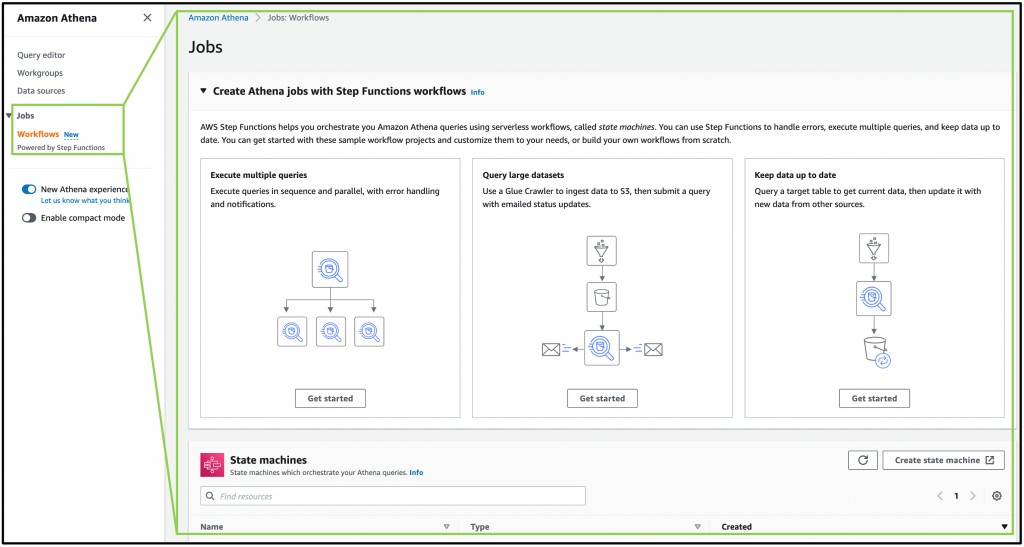
Using Athena query patterns from Step Functions
Execute multiple queries
In Athena, you run SQL queries in the Athena console against Athena workgroups. With Step Functions, you can run Athena queries in a sequence or run independent queries simultaneously in parallel using a parallel state. Step Functions also natively handles errors and retries related to Athena query tasks.
Workflow orchestration in the Athena console provides these capabilities to run and visualize multiple queries in Step Functions. For example:
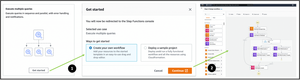
- Choose Get Started from Execute multiple queries.
- From the pop-up, choose Create your own workflow and select Continue.
A new browser tab opens with the Step Functions Workflow Studio. The designer shows a workflow pattern template pre-created. The workflow loads data from a data source running two Athena queries in parallel. The results are then published to an Amazon SNS topic.
Alternatively, choosing Deploy a sample project from the Get Started pop-up deploys a sample Step Functions workflow.
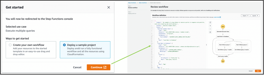
This option creates a state machine. You then review the workflow definition, deploy an AWS CloudFormation stack, and run the workflow in the Step Functions console.
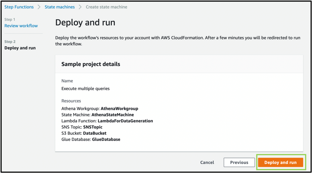
Once deployed, the state machine is visible in the Step Functions console as:

Select the AthenaMultipleQueriesStateMachine to land on the details page:
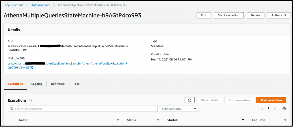
The CloudFormation template provisions the required AWS Glue database, S3 bucket, an Athena workgroup, the required AWS Lambda functions, and the SNS topic for query results notification.
To see the Step Functions workflow in action, choose Start execution. Keep the optional name and input and choose Start execution:
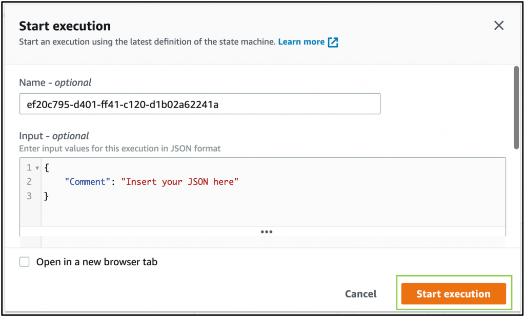
The state machine completes the tasks successfully by Executing multiple queries in parallel using Amazon Athena and Sending query results using the SNS topic:
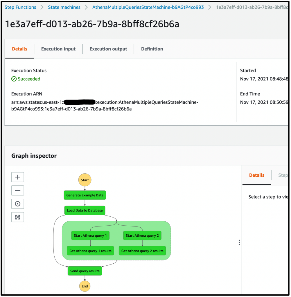
The state machine used the Amazon Athena StartQueryExecution and GetQueryResults tasks. The Workflow orchestration in Athena console now highlights this newly created Step Functions state machine:
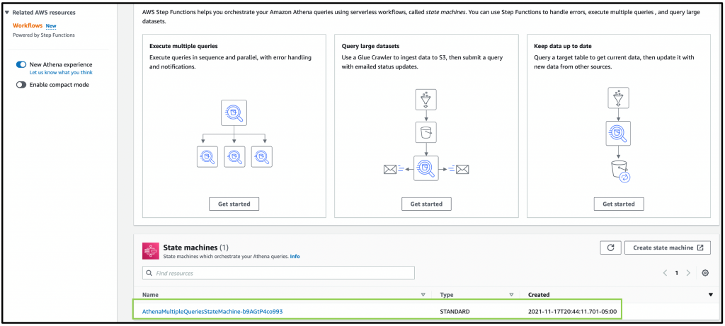
Any state machine that uses this task in Step Functions in this account is listed here as a state machine that orchestrates Athena queries.
Query large datasets
You can also ingest an extensive dataset in Amazon S3, partition it using AWS Glue crawlers, then run Amazon Athena queries against that partition.
Select Get Started from the Query large datasets pop-up, then choose Create your own workflow and Continue. This action opens the Step Functions Workflow studio with the following pattern. The Glue crawler starts and partitions large datasets for Athena to query in the subsequent query execution task:
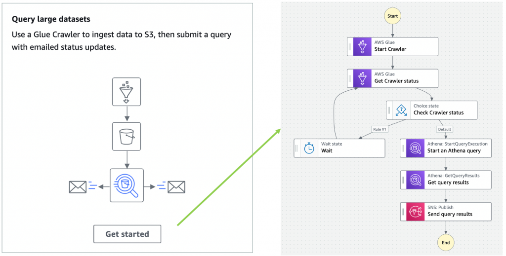
Step Functions allows you to combine Glue crawler tasks and Athena queries to partition where necessary before querying and publishing the results.
Keeping data up to date
You can also use Athena to query a target table to fetch data, then update it with new data from other sources using Step Functions’ choice state. The choice state in Step Functions provides branching logic for a state machine.

You are not limited to the previous three patterns shown in workflow orchestration in the Athena console. You can start from scratch and build Step Functions state machine by navigating to the bottom right and using Create state machine:
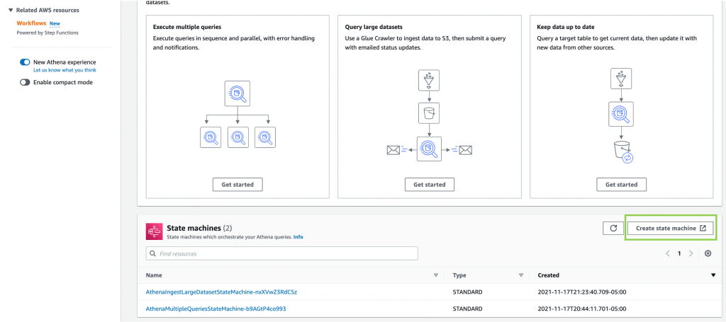
Create State Machine in the Athena console opens a new tab showing the Step Functions console’s Create state machine page.

Refer to building a state machine AWS Step Functions Workflow Studio for additional details.
Step Functions integrates with all Amazon Athena’s API actions
In September 2021, Step Functions announced integration support for 200 AWS services to enable easier workflow automation. With this announcement, Step Functions can integrate with all Amazon Athena API actions today.
Step Functions can automate the lifecycle of an Athena query: Create/read/update/delete/list workGroups; Create/read/update/delete/list data catalogs, and more.
Other AWS service integrations
Step Functions’ integration with the AWS SDK provides support for 200 AWS Services and over 9,000 API actions. Athena tasks in Step Functions can evolve by integrating available AWS services in the workflow for their pre and post-processing needs.
For example, you can read Athena query results that are put to an S3 bucket by using a GetObject S3 task AWS SDK integration in Step Functions. You can combine different AWS services into a single business process so that they can ingest data through Amazon Kinesis, do processing via AWS Lambda or Amazon EMR jobs, and send notifications to interested parties via Amazon SNS or Amazon SQS or Amazon EventBridge to trigger other parts of their business application.
There are multiple ways to decorate around an Amazon Athena job task. Refer to AWS SDK service integrations and optimized integrations for Step Functions for additional details.
Important considerations
Workflow orchestrations in the Athena console only show Step Functions state machines that use Athena’s optimized API integrations. This includes StartQueryExecution, StopQueryExecution, GetQueryExecution, and GetQueryResults.
Step Functions state machines do not show in the Athena console when:
- A state machine uses any other AWS SDK Athena API integration task.
- The APIs are invoked inside a Lambda function task using an AWS SDK client (like Boto3 or Node.js or Java).
Cleanup
First, empty DataBucket and AthenaWorkGroup to delete the stack successfully. To delete the sample application stack, use the latest version of AWS CLI and run:
aws cloudformation delete-stack --stack-name <stack-name>
Alternatively, delete the sample application stack in the CloudFormation console by selecting the stack and choosing Delete:
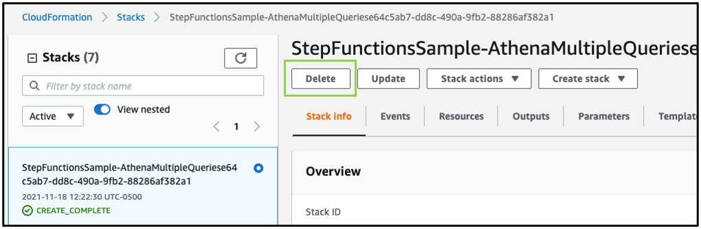
Conclusion
Amazon Athena console now provides an integration with AWS Step Functions’ workflows. You can use the provided patterns to create and visualize Step Functions’ workflows directly from the Amazon Athena console. Step Functions’ workflows that use Athena’s optimized API integration appear in the Athena console. To learn more about Amazon Athena, read the user guide.
To get started, open the Workflows page in the Athena console. Select Create Athena jobs with Step Functions Workflows to deploy a sample project, if you are new to Step Functions.
For more serverless learning resources, visit Serverless Land.
Page 1|Page 2|Page 3|Page 4